WideDTA:Way to predict Drug-target binding affinity using CNN in Drug Discovery Process-Model2
** Discovery of potential drugs for new targets is an expensive and time consuming process so we can use deep learning in the pipeline of drug-discovery to save the time and cost.** In previous blog:(this ),I wrote about use of deep learning architecture in identification of drug-target interactions (DTI) strength (binding affinity) using character-based sequence representation approach.
The successful identification of drug–target interactions (DTI) is a critical step in drug discovery. As the field of drug discovery expands with the discovery of new drugs, repurposing of existing drugs and identification of novel interacting partners for approved drugs is also gaining interest.
The protein–ligand interactions assume a continuum of binding strength values, also called binding affinity and we are predicting this value using deep learning architectures.Furthermore, a regression-based model brings in the advantage of predicting an approximate value for the strength of the interaction between the drug and target which in turn would be significantly beneficial for limiting the large compound search-space in drug discovery studies.
In this model, I used the word-based sequence representation. it is a promising alternative to the character-based sequence representation approach (previous blog)in deep learning models for binding affinity prediction.
Dataset and Data Preprocessing- We evaluated our model on the KIBA data set (kinase inhibitors bioactive data).We used the filtered version of the KIBA dataset, in which each protein and ligand has at least ten interactions. KIBA set contains ligands-2111, and proteins-229.
In this we have different lengths of proteins and ligands ,But we considered ligand have sequence length 50(characters) and for every protein sequence is 600(characters)number of proteins and ligands reduced this is easy to run in my CPU.If We have GPU we can take max length to consider more number of proteins and ligands.
Here, we used three different text-based information sources to model. In previous blog work showed that the use of protein sequence and ligand SMILES is an effective approach to model the interactions between these entities .In this work, we explored the effect of adding additional specific information, namely domain/motif information for the proteins , which might contribute to a better modeling of the interactions.
The input to the model is-three seq. LS,PS,PDM
Protein Sequence (PS) - The protein sequence is composed of 20 different types of amino acids. We first collected the sequences of the respective proteins for each dataset and then, extracted 3-residue words from the sequences. For instance, an example protein Kinase SGK1 (UniProt, O00141) with the sequence of “MTVKTEAAKGTLTYSRMRGMVA……YAPPTDSFL” is represented with the following set of words { ‘MTV’, ‘KTE’, …, ‘TDS’, ‘TVK’, ‘TEA’, …, ‘DSF’, ‘VKT’, ‘EAA’, …, ‘SFL’}.
Protein Domains and Motifs (PDM) - PROSITE is database that serves as a resource for motif and profile descriptors of the proteins . Multiple sequence alignment of protein sequences reveals that specific regions within the protein sequence are more conserved than others, and these regions are usually important for folding, binding, catalytic activity or thermodynamics. These subsequences are called either motifs or profiles. A motif is a short sequence of amino-acids (usually 10–30 ), while profiles provide a quantitative measure of sequences based on the amino-acids they contain. Profiles are better at detection of domains and families. For instance, Kinase SGK1 (UniProt, O00141) has the ATP-binding motif ‘IGKGSFGKVLLARHKAEEVFYAVKVLQKKAILK’, while the Protein Kinase Domain profile is about seven times longer than the motif. We used the PROSITE database to extract motifs and profiles for each respective protein in our datasets. We then extracted 3-residue subsequences from each motif and domain similarly to the approach adopted in PS.
Ligand SMILES (LS)- A chemical compound can be represented with a SMILES string refer this ), the SMILES string “C(C1CCCCC1)N2CCCC2” is divided into the following 8-character chemical words: “C(C1CCCC”, “(C1CCCCC”, “C1CCCCC1”, “1CCCCC1), “CCCCC1)N”, “CCCC1)N2”, … ,”)N2CCCC2”.We experimented with word length ranging between the values of 7–12 and there was no statistically significant difference in the prediction performance, therefore we choose 8 to be the character length.
We modified the syntax of SMILES representation, into Deep SMILES .Deep SMILES modifies the use of parentheses and ring closure digits in the regular SMILES and aims to enhance the performance of the machine learning algorithms that employ SMILES notation as input in various different tasks. We first extracted the canonical SMILES of the compounds from PubChem , and then converted each SMILES to DeepSMILES . For instance the SMILES string “C(C1CCCCC1)N2CCCC2” is represented as “CCCCCCC6))))))NCCCC5” and the chemical words are: “CCCCCCC6”, “CCCCCC6)”, “CCCCC6))”, … , “))NCCCC5” with Deep SMILES.
We build a word-based model instead of a character based model because of this reasons: (i) motifs and domains that were extracted from a protein sequence were not sequential and they can contain overlapping residues.
Input representation to the model: We used one-hot encoding for the ligand (characters) ,protein (characters) and motif to represent inputs. Since Both SMILES (Len<50) and protein sequences (Len<600) have varying lengths. Hence, in order to create an effective representation form (one-hot representation), we decided on fixed maximum lengths of 50 for SMILES and 600 for protein sequences for our dataset.For more details refer this(article on Github:refer this ).
Custom Dataset - We implemented the Custom Dataset and used Pytorch Dataloader-torch.utils.data.DataLoader to access the dataset .Built the separate train and test loader for training and testing the model.
import torch
from torch.utils.data import Dataset
class widedata(Dataset):
    def __init__(self,ligand_path,protein_path,keys,motif_path,affinity_path):
       with open(ligand_path) as ligand_data:
           self.lig=ps(deepsml(filter(json.load(ligand_data),20)),8)
           self.lig2=onehot(self.lig)
           #print(self.lig2)
            ##remain torch tnsr
       with open(protein_path) as protein_data:
           self.pro=filter(json.load(protein_data),600)
           list(map(self.pro.pop, keys))
           self.pro=ps((self.pro),3)
           self.pro2=onehot(self.pro)
            ##torch tnsr remain
       with open(motif_path) as motif_data:
           self.motif =ps(json.load(motif_data),3)
           self.moti2 =onehot(self.motif)
           ##tnsr
       with open(affinity_path,'rb') as Y:
          self.y = torch.Tensor(np.nan_to_num(pickle.load(Y, encoding='latin1')))
          #self.y = np.nan_to_num(pickle.load(Y,encoding='latin1'))
          self.mpmy=MPMy(self.lig2,self.pro2,self.moti2,self.y)
    def __len__(self):

        return len(self.mpmy)

    def __getitem__(self, idx):
        return self.mpmy[idx]
dataset = widedata(ligand_path, protein_path,keys,motif_path,affinity_path)
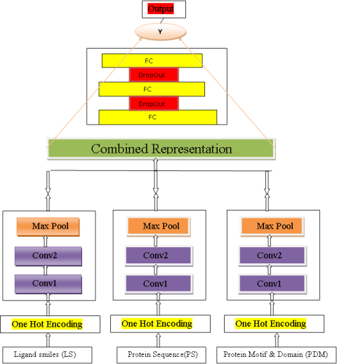
PREDICTION MODEL- We built a CNN-based model in Pytorch library, which we call WideDTA, that combines at most three pieces of different textual information. architecture of model is similar to the CNN-based (DeepDTA blog on Github:refer this ). The difference is that DeepDTA is a character based model, whereas WideDTA depends on words as input.
Model Architecture- In our CNN Model, for each text-based information module, we used two 1D-convolutional layers with a max pooling layer on top and Rectified Linear Unit (RELU) as the activation function. We used 16 filters in the first CNN layer and 32 in the second CNN layer in order to capture more specific patterns.
We followed this architecture and built three separate CNN Block for protein sequence, ligands, and motif/domain information. Features extracted from these blocks were concatenated and fed into three fully connected layers , which had two drop-out layers in between (value of 0.3) to prevent over-fitting.
import torch
import torch.nn as nn
import data_w
from data_w import*
from torch import optim
import torch.nn.functional as F
class WideCNN(nn.Module):
     def __init__(self):
         super().__init__()
         ###protein
         self.pconv1=nn.Conv1d(in_channels=6729, out_channels=16, kernel_size=2, stride=1, padding=1)
         self.pconv2=nn.Conv1d(16,32,2,stride=1, padding=1)
         self.maxpool=nn.MaxPool1d(2,2)
         ###ligands
         self.lconv1=nn.Conv1d(in_channels=10,out_channels=16,kernel_size=2,stride=1,padding=1)
         self.lconv2=nn.Conv1d(16,32,2,stride=1,padding=1)
         #####motif
         self.mconv1=nn.Conv1d(in_channels=1076,out_channels=16,kernel_size=2,stride=1,padding=1)
         self.mconv2=nn.Conv1d(16,32,2,stride=1,padding=1)

         self.dropout=nn.Dropout(.3)
         self.FC1=nn.Linear(5120,512)
         self.FC2=nn.Linear(512,10)
         self.FC3=nn.Linear(10,1)
     def forward(self,x1,x2,x3):
         x1=self.maxpool(F.relu(self.pconv1(x1)))
         x1=self.maxpool(F.relu(self.pconv2(x1)))

         x2=self.maxpool(F.relu(self.lconv1(x2)))
         x2=self.maxpool(F.relu(self.lconv2(x2)))

         x3=self.maxpool(F.relu(self.mconv1(x3)))
         x3=self.maxpool(F.relu(self.mconv2(x3)))
         x1=x1.view(-1,149*32)
         x2=x2.view(-1,3*32)
         x3=x3.view(-1,8*32)
         x=torch.cat([x1,x2,x3],1)
         x = F.relu(self.FC1(x))
         x = self.dropout(x)
         x = F.relu(self.FC2(x))
         x = self.dropout(x)
         x = self.FC3(x)
         return x

modelw=WideCNN()
modelw
if __name__ == '__main__':
    print(modelw)
For training the Model we have used Adam Optimizer and RMSE loss.(For full code on Github:visit this )
This is a deep-learning based approach to predict drug-target binding affinity, which we refer to as WideDTA. I hope you enjoyed coding up with Deeplearning.